1 . HOW TO CRATE TABLE IN EXCEL

Introduction

This article has been published on the Microsoft site (in Dutch)
With the release of Excel 2007, Microsoft has introduced a new concept of working with tables of data. This new functionality is (not surprisingly) called "Tables". In fact, Tables in Excel 2007 are the successor of Excel 2003's "List" feature, with added functionality.
This article introduces you into the concepts of working with Tables in Excel 2013, 2010 and 2007 and shows you how they may help you in your everyday Excel use.

Creating Your Table

Creating a table in Excel is easy. Of course you already have some data available somewhere on your sheet. Select the cells that contain the data:

Figure 1: Select the table area
Next, on the Home tab of the ribbon, find the group called "Styles". Click on the button that says "Format as Table" (see figure 2):

Figure 2: "Format as Table" button on the Styles group of the Home tab.
After clicking this button, Excel shows a new user interface element called a gallery, with a number of formatting choices for your table, see figure 3:

Figure 3: Table format gallery.
Select one of the predetermined formats. After clicking one of the formats, Excel will ask you what range of cells you want to convert to a table (see figure 4). If your table contains a heading row, make sure the checkbox is checked. Click OK to convert the range to a table.

Figure 4: Dialog asking what range of cells has to be converted to a table.
After you’ve finished these steps, your table will look like figure 5.

Figure 5: Range of cells, after converting to table

Special functionality of a Table

After defining a table, the area gains special functionalities:

1. Integrated autofilter and sort functionality

If your Table has a header row, it will always have filter and sorting dropdowns in place on the header row. See figure 6:

Figure 6: sorting and filtering dropdowns

2. Easy selecting

Selecting an entire column or row is simple: move your mouse to the top of the table until the pointer changes to a down pointing arrow (figure 7) and click. The data area of that column is selected. Click again to include the header and total rows in the selection.

Figure 7: selecting an entire column of data within your table
You can also select the entire data area or the entire table by clicking near the table’s top-left corner (the mousepointer changes to a south-east pointing arrow, see figure 8).

Figure 8: selecting all data within your table or the whole table is just one or two clicks away.

3. Header row remains visible whilst scrolling

If your table is larger than fits on a screen and you scroll down, Excel 2007 has a nice new feature: the column letters are temporarily replaced with the table’s column names (but only whilst you’re inside the table!). See figure 9.

Figure 9: Table header names on Excel’s column header when scrolling

4. Automatic expansion of table

If you type anything next to a table, Excel assumes you want to expand the table and automatically increases the table size to include your new entry. Of course you can undo this expansion too, or switch off this behavior entirely.

5. Automatic reformatting

When you insert or remove a row (or column) in your table, Excel will automatically adjust the formatting: alternate shading is kept nicely in place.

6. Automatic adjustment of charts and other objects source range

If you add rows to your table, any object that uses your table’s data will automatically include the new data.

Table Options on the Ribbon

Once you have selected any of the cells within the table, you will see a new tab appear on the ribbon, called Table Tools, Design. Figure 10 shows you what the ribbon will look like after you click this tab.

Figure 10: Ribbon after clicking the Table Tools tab.
Each group on this tab is discussed in the following paragraphs.

Properties group

The properties group (see figure 11 below) enables you to do two things:

Figure 11: properties group on Table Tools tab

1. change the Name of the table

The name of a table is used when you refer to cells within the table in a formula.

2. Change the size of the table

Click this control to change the size of your table.

Tools group

This group (see figure 12) has three controls:

Figure 12: Tools group on Table Tools tab

1. Summarize with PivotTable

It is obvious what this control does. After you have created the pivot table, you don’t need to worry about updating the sourcerange of the pivot table anymore. If you add data to your table, Excel automatically expands the source range of the Pivot table to reflect your changes. Of course you still have to refresh the Pivot table to see the results.

2. Remove Duplicates

Another new feature which has been added to Excel 2007. After clicking this control, you are presented with a dialog with which you can select the columns that you want to use to determine whether a row in the table is unique. (see figure 13)

Figure 13: Remove Duplicates dialog

3. Convert to Range

By pressing this button you demote the table back to a normal range. Beware if you do this when you’ve based e.g. a pivot table on the range, the Pivot table’s source range will not be updated and the pivot table cannot be refreshed anymore.

The External Table Data Group

This group (shown in figure 14) is all about the source data of a table and only applies if the data in the table has been imported into Excel using a database- or webquery or a sharepoint list.

Figure 14: External Table Data group on the Table Tools tab of the ribbon
This group has 5 buttons:

1. Export Data

This is in fact a combobutton. If you press it you’re offered two options,
"Export Table to SharePoint List" and "Export Table to Visio PivotDiagram". What these are exactly is beyond the scope of this article.

2. Refresh

Use this combobutton to refresh the external data in your table. If you click the arrow beneath the button, you’re offered a menu which amongst others also includes "Refresh All", with which you can refresh all external data ranges in your file.

3. Data Range Properties

This button can be used to change the properties of the external data you have based your table on.

4. Open in Browser

If your table is a sharepoint list, this button enables you to open a browser window with that list.

5. Unlink

If your table is a sharepoint list, this button disconnects the table from the list.

Table Style Options Group

This group houses the controls which determine how table styles are applied to your table (see figure 15).

Figure 15: Table Style Options group on the Table Tools tab of the ribbon

1. Header Row

When this box is unchecked, Excel removes the header row from your table. The cells of the header row are cleared, but Excel does remember the header. If you type anything into any cell in that now empty row, Excel will not overwrite that information when you check the box again. Instead, Excel will insert a new row to show the header. Cells below the table are then moved down.

2. Total Row

Check this box if you want a total row below your table. Excel will automatically add a sum function below the last column in your table.

3. Banded Rows

Check this box to get alternating shading for the rows in your table.

4. First Column

If you check this box, the first column of your table will be formatted differently from the other columns.

5. Last Column

Formats the last column of your table differently from the other columns.

6. Banded Columns

Check this box to get alternating shading for the columns in your table

Table Styles Group

The last group on the Table Tools tab enables you to quickly change the style of your table (see figure 16).

Figure 16: Table Styles group on the Table Tools tab of the ribbon
Click the dropdown button to the right of the gallery to see all choices available to you. Hover over a particular style to see what your table would look like when you click it. At the bottom of the gallery there are two extra choices:

1. New Table Style

This option enables you to create your own table style.

2. Clear

Use this to remove the table style from your table entirely. Number formats are retained.

Referencing cells in a table (structured referencing)

Excel 2007 introduces a new syntax to refer to cells inside a table. To see how this works, click in a cell to the immediate right of the table, hit the = sign, type SUM( and then click on any cell with data within the table. You’ll get a formula like this one:
Excel 2007: =SUM(Table3[[#This Row];[Discount]])
This syntax has been simplified in Excel 2010 and 2013:
=SUM(Table3[@Discount])
The new naming convention to refer to the cells in your table works as follows:
Table3: The name of your table
[#This Row] in Excel 2007, @ in Excel 2010-2013 : Denotes the data comes from the same row your formula cell is in
[Discount] : The column inside the table
Some other examples:

Description	Excel 2007	Excel 2010, 2013
The entire table	=Table1	=Table1
The same row in the table	=Table1[[#This Row][Discount]]	=Table1[@Discount]
Heading of table	=Table1[#Headers]	=Table1[#Headers]
Entire table (2)	=Table1[#All]	=Table1[#All]
Table total row	=Table1[#Totals]	=Table1[#Totals]

2 . GIVE EXAMPLE FOR MATHEMATICS FORMULA USING EXCEL

How to Change Relative Formulas to Absolute Formulas in Excel 2013

By Greg Harvey from Excel 2013 For Dummies

All new you create in Excel 2013 naturally contain relative references unless you make them absolute. Because most copies you make of formulas require adjustments of their cell references, you rarely have to give this arrangement a second thought. Then, every once in a while, you come across an exception that calls for limiting when and how cell references are adjusted in copies.
One of the most common of these exceptions is when you want to compare a range of different values with a single value. This happens most often when you want to compute what percentage each part is to the total.
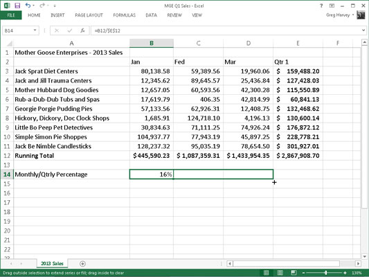
For example, in the Mother Goose Enterprises – 2013 Sales , you encounter this situation in creating and copying a formula that calculates what percentage each monthly total (in the cell range B14:D14) is of the quarterly total in cell E12.

Suppose that you want to enter these formulas in row 14 of the Mother Goose Enterprises – 2013 Sales worksheet, starting in cell B14. The formula in cell B14 for calculating the percentage of the January-sales-to-first-quarter-total is very straightforward:

=B12/E12

This formula divides the January sales total in cell B12 by the quarterly total in E12 (what could be easier?). Look, however, at what would happen if you dragged the fill handle one cell to the right to copy this formula to cell C14:

=C12/F12

The adjustment of the first cell reference from B12 to C12 is just what the doctor ordered. However, the adjustment of the second cell reference from E12 to F12 is a disaster. Not only do you not calculate what percentage the February sales in cell C12 are of the first quarter sales in E12, but you also end up with one of those horrible #DIV/0! error things in cell C14.
To stop Excel from adjusting a cell reference in a formula in any copies, convert the cell reference to absolute. To do this, press the key F4, after you apply Edit mode (F2). You make the cell reference absolute by placing dollar signs in front of the column letter and row number. For example, cell B14 contains the correct formula to copy to the cell range C14:D14:

=B12/$E$12

Look at the worksheet after this formula is copied to the range C14:D14 with the fill handle and cell C14 is selected. Notice that the shows that this cell contains the following formula:

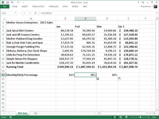
=C12/$E$12

Because E12 was changed to $E$12 in the original formula, all the copies have this same absolute (non-changing) reference.

If you goof up and copy a formula where one or more of the cell references should have been absolute but you left them all relative, edit the original formula as follows:

Double-click the cell with the formula or press F2 to edit it.
Position the insertion point somewhere on the reference you want to convert to absolute.
Press F4.
When you finish editing, click the Enter button on the Formula bar and then copy the formula to the messed-up cell range with the fill handle.

Be sure to press F4 only once to change a cell reference to completely absolute. If you press the F4 function key a second time, you end up with a so-called mixed reference, where only the row part is absolute and the column part is relative (as in E$12).

If you then press F4 again, Excel comes up with another type of mixed reference, where the column part is absolute and the row part is relative (as in $E12). If you press F4 yet again, Excel changes the cell reference back to completely relative (as in E12). After you’re back where you started, you can continue to use F4 to cycle through this same set of cell reference changes.
If you’re using Excel on a touchscreen device without access to a physical keyboard, the only way to convert in your formulas from relative to absolute or some form of mixed address is to open the Touch keyboard and use it add the dollar signs before the column letter and/or row number in the appropriate cell address on the Formula bar

3 . HOW TO INSERT SYMBOL RM WITH 2 DECIMAL PLACES

Find out the Check Mark Symbol at ease if you have Classic Menu for Office

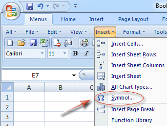
Figure 1: Symbols in Classic Menu

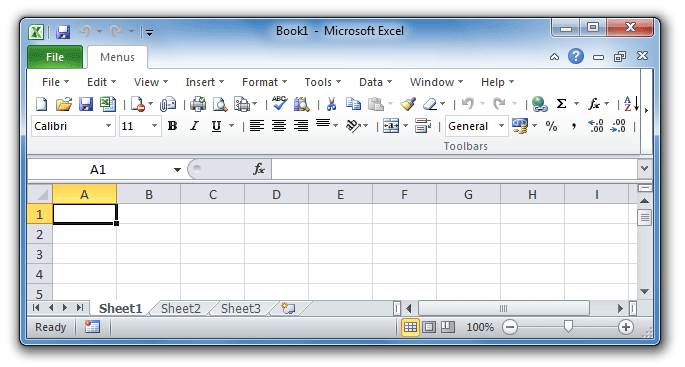
Classic Menu for Office enable all your use habit adopted in Excel 2003/XP(2002)/2000 are valid in Excel 2007/2010/2013.

Step 1: Click the Menus tab;
Step 2: Click the Insert drop down menu
Step 2: Find out the Symbol item.

The Figure 1 and Figure 2 may help you more.

Step 3: Click the Symbol item, then you will view : the Symbol dialog box; the figure 2 may help you follow these steps easily.
Step 5: Click the Symbols tab;
Step 6: Select the Wingdings from the Font drop down box;
Step 7: Move the Scroll bar to the bottom, and you will view the Check Mark symbols.

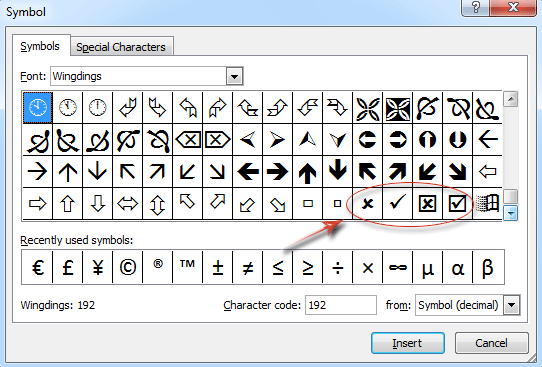
Figure 2: Symbols dialog box

More Classic Menu for Office...

Find out the Check Mark Symbol in Ribbon if you do not have Classic Menu for Office

Click the Insert tab;
Go to Text group;
Click the Symbol button;

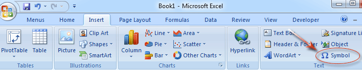
Figure 3: Symbols button in Ribbon

After clicking the symbol button, you will enter the Symbol dialog box. You can just follow the steps we mentioned above to find out the Check Mark Symbols.

More Tips for Microsoft Excel 2007, 2010 and 2013

Classic Menu for Office

Brings the familiar classic menus and toolbars back to Microsoft Office 2007, 2010 and 2013. You can use Office 2007/2010/2013 immediately without any training. Supports all languages, and all new commands of 2007, 2010 and 2013 have been added into the classic interface.

		Classic Menu for Office 2010 and 2013 It includes Classic Menu for Word, Excel, PowerPoint, OneNote, Outlook, Publisher, Access, InfoPath, Visio and Project 2010 and 2013.
		Classic Menu for Office 2007 It includes Classic Menu for Word, Excel, PowerPoint, Access and Outlook 2007.

Conclusion

I used less versed in the field of IT but now I've been smart to excel